
How VectorDBs Work Internally + How To Make The Most Out Of Them
What's really happening when you do vector search, and how to take advantage of that to improve retrieval accuracy.

Introduction
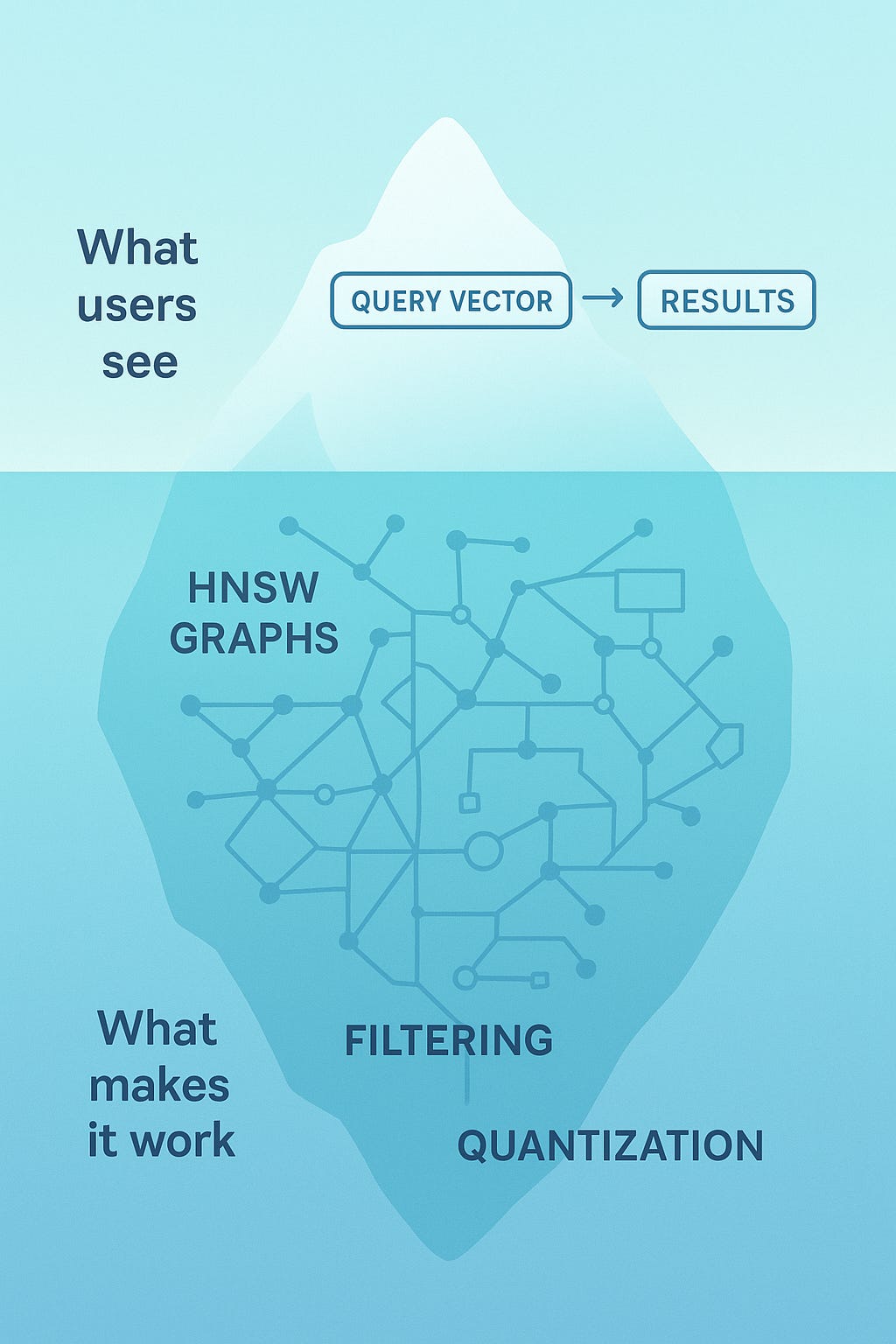
VectorDBs like Pinecone, ChromaDB, Qdrant, etc. are often described as comparing a query vector against all stored vectors with cosine similarity and then returning the top k results.
BUT that’s not how any production vector database actually works. If it did, queries would take seconds or minutes instead of milliseconds. The reality is far more interesting, and understanding it will change how you think about building with vector databases.
List of Contents
The Naive Approach – Brute-force search limitations explained clearly
Distance Concentration in High Dimensions – Why high-dimensional spaces behave strangely + efficient alternatives to linear search
HNSW Algorithm – Navigable graphs for fast search
Other Indexing Strategies – IVF, PQ, LSH tradeoffs explored
Tradeoffs in Vector Databases – Balancing recall, speed, memory usage
RAG Patterns and VectorDBs – How different pipelines use databases
Production Realities – Filtering, updates, sharding, latency challenges
Implications for Applications – Designing systems around query patterns
The Naive Approach and Why High Dimensions Break Everything
Let’s start with the naive approach. You have a million documents embedded as 1536-dimensional vectors (thanks, OpenAI). A query comes in, also a 1536-dimensional vector. The database compares your query against all million vectors, computes the cosine similarity for each, sorts them, and returns the top 10.
This is called a linear scan or brute force search, and it’s O(n) in complexity. For a million vectors with 1536 dimensions each, that’s over 1.5 billion floating-point operations per query. Even on modern hardware, this doesn’t scale.
But there’s a deeper problem: high-dimensional spaces are profoundly weird.
In 2D or 3D space, your intuition works. Close points are close, far points are far. Neighbourhoods make sense. But as you add dimensions, strange things happen. The volume of a hypersphere becomes concentrated in a thin shell near its surface. Points become roughly equidistant from each other. The concept of “nearest neighbor” starts to lose meaning because everything is roughly the same distance away.
This is called distance concentration, and it’s why techniques that work in low dimensions fail spectacularly in high dimensions. You can’t just partition space naively—you need fundamentally different approaches.
The key insight: vector databases don’t actually find the true nearest neighbours. They find approximate nearest neighbours, and they do it using clever data structures that exploit the structure of high-dimensional spaces.
HNSW (Hierarchical Navigable Small World)
HNSW is the algorithm that powers most modern vector databases, and it’s based on a brilliant insight: searching high-dimensional spaces is like navigating a social network.
Think about the “six degrees of separation” phenomenon. Even in a network of billions of people, you can reach anyone through a short chain of connections. The network is a “small world”—high clustering (your friends know each other) but short path lengths to anyone.
HNSW builds a navigable version of this for vectors.

How the layers work
HNSW constructs multiple layers of proximity graphs. Each layer is a graph where nodes are vectors and edges connect similar vectors. The key properties:
Layer 0 (bottom): Contains all vectors, densely connected
Higher layers: Contain exponentially fewer vectors, acting as “express lanes”
Each vector appears in layer 0 and potentially in higher layers (chosen probabilistically)
When you insert a vector, the algorithm randomly assigns it a layer (using an exponential decay distribution—most vectors stay in layer 0, few reach high layers). Then it connects the vector to its nearest neighbors in each layer it occupies.
Searching the graph
To find nearest neighbors for a query:
Start at the highest layer with the entry point (a designated vector)
Greedily traverse to closer and closer vectors (friends-of-friends search)
When you can’t get closer, descend to the next layer
Repeat until you reach layer 0
At layer 0, explore more thoroughly to find the final nearest neighbors
The greedy traversal is key: at each step, you look at your neighbours’ neighbours and move to whoever is closest to the query. This works because the graph structure ensures you’re making progress toward the true nearest neighbours.
You search logarithmically instead of linearly. For a million vectors, you might only visit a few hundred during the search instead of all million!!!
Other Indexing Strategies
HNSW isn’t the only method. Different algorithms make different tradeoffs:
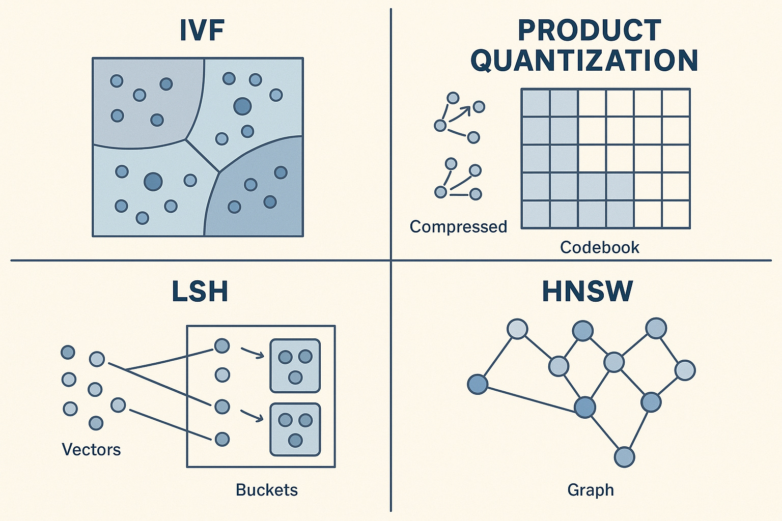
IVF (Inverted File Index): Partition your vector space into clusters (using k-means or similar). At query time, find the nearest cluster centroids, then only search within those clusters. Fast queries, but accuracy depends on how well your data clusters. Think of it like searching specific file drawers instead of the whole filing cabinet.
Product Quantisation: Compress your vectors by splitting each into subvectors and quantising each subvector to a codebook. Store codes instead of full vectors. Massive memory savings (10-100x compression) but lossy. You’re essentially storing a compressed “sketch” of each vector.
LSH (Locality-Sensitive Hashing): Hash vectors such that similar vectors collide in the same buckets with high probability. Query by hashing and checking buckets. Probabilistic guarantees but simpler to implement. Works well for binary or lower-dimensional vectors.
When to use what:
HNSW is the default for most use cases—excellent recall and speed, reasonable memory usage. IVF when you have natural clusters or need extreme speed at the cost of some accuracy. Product Quantization when memory is your bottleneck. LSH for specialized cases or when you need theoretical guarantees.
The Tradeoffs To Always Remember
Vector databases live in a three-way tradeoff space: recall (accuracy), speed, and memory. You can’t have all three maxed out.
Recall vs. speed: HNSW has parameters like ef_construction (neighboUrs to consider during building) and ef_search (neighboUrs to consider during querying). Higher values = better recall but slower queries. In production, 95% recall might be perfectly fine and 10x faster than 99% recall.
Build time vs. query time: HNSW is expensive to build—you’re constructing multiple graph layers. IVF is cheaper to build but may require more work at query time. This matters: if you’re reindexing frequently, build time dominates.
Why “approximate” matters (and when it doesn’t): The “approximate” in ANN (Approximate Nearest Neighbor) search means you might not get the true top-k results. You might get the 1st, 3rd, 5th, 8th, and 12th nearest neighbours instead of the 1st through 5th. For RAG applications, this usually doesn’t matter—your retrieval is approximate anyway, and the LLM is robust to minor variations in context. For face recognition or deduplication, you might need higher recall.
The dirty secret: most applications never measure their recall. They tune parameters based on vibes and latency budgets, not actual accuracy metrics.
How Different RAG Patterns Actually Use VectorDBs
Here’s where it gets interesting: not all RAG is created equal, and different patterns stress vector databases differently.
Naive RAG is what most people start with: embed the query, fetch top-k chunks, stuff them into context. Simple top-k retrieval, single query per request. This is the “happy path” all vector databases optimise for.
Hybrid search combines dense vectors (embeddings) with sparse vectors (BM25 or keyword features). Your database needs to maintain two separate indices and somehow merge the results. Some systems do this natively (Weaviate, Elasticsearch), others require you to query twice and merge in application code. The vector index does semantic search while a traditional inverted index handles keywords, then you combine scores with something like reciprocal rank fusion.
HyDE (Hypothetical Document Embeddings) flips the script: instead of embedding your query, you use an LLM to generate a hypothetical answer, then embed that and search. Why? Because your query “What causes inflation?” embeds differently than document text “Inflation is caused by excessive money supply growth relative to economic output.” HyDE bridges this gap. From the vector DB’s perspective, it’s still just a query vector, but the query pattern changes—you’re doing more preprocessing before you hit the database.
Reranking pipelines over-fetch from the vector database (maybe top-100 instead of top-10), then use a cross-encoder or LLM to rerank. The vector database does coarse retrieval—fast but approximate—then a more expensive model does fine-grained relevance scoring. This means your vector database queries are actually less critical: you’re optimizing for recall over precision since the reranker will fix ordering later.
Agentic/iterative RAG involves multiple queries: the agent might search, read results, reformulate the query, search again. This creates bursty query patterns. Instead of one query per user request, you might do 3-10. Latency compounds, and p99 latencies matter more because a slow query in the chain stalls everything.
Graph RAG uses the vector database as an entry point, not the final answer. You vector search to find a starting node, then traverse a knowledge graph. The vectorDB needs to return not just vectors but associated graph IDs/metadata for the graph traversal. Filtering becomes critical here (more on that below).
Your query patterns determine what you need from your infrastructure. Naive RAG can tolerate higher latency and single-shot queries. Agentic RAG needs consistently low latencies. Hybrid search needs multiple index types. Reranking pipelines need high throughput more than perfect accuracy.
Production Realities
Now for some issues that you’ll face in production:
Filtering
You want to search vectors but only among documents from a specific user, or published after a certain date, or tagged with certain categories. This is called metadata filtering, and it destroys performance.
Why? Because HNSW (and most other indices) is built assuming you’re searching the entire dataset. When you add a filter, you’re searching a subset. But the graph structure doesn’t know about your subset—it still needs to traverse the full graph, checking each candidate against your filter. You might visit 100 nodes to find 10 that match your filter.
Some databases handle this better than others. Native metadata indexing, pre-filtering strategies, separate indices per filter value—all have tradeoffs. The brutal truth: heavily filtered queries can be 10-100x slower than unfiltered ones.
Updates and deletes
Vector databases are optimized for write-once, read-many workloads. Updates and deletes are painful.
Deleting a vector means finding it in the graph and removing it, which leaves the graph structure degraded. You might have “orphan” regions with poor connectivity. Most databases mark vectors as deleted rather than actually removing them, then periodically rebuild indices.
Updates are worse: you need to delete and reinsert, which means removing edges and creating new ones. Do this frequently and your graph degrades.
The practical implication is that vector databases are not OLTP systems. If you need frequent updates, batch them. If you need real-time updates, expect performance degradation or plan for regular reindexing.
Sharding and distributed search
Once you outgrow a single machine, you need to shard. But vector search doesn’t partition cleanly like SQL databases.
You can’t just hash vectors and search each shard independently—nearest neighbours might be on different shards. Most systems use one of two approaches:
Search all shards in parallel and merge results. Simple but latency is determined by the slowest shard (p99 becomes critical).
Partition using clustering (like IVF at the shard level) and route queries to relevant shards. Better performance but complex and can miss results if the partitioning is poor.
Replication helps with throughput but doesn’t solve the fundamental problem: vector search is globally interconnected in a way that row-based data isn’t.
Cold start problems
HNSW graphs work best when hot in memory. A cold database might need to page in large portions of the graph during the first queries, causing huge latency spikes. Preheating or keeping indices warm is essential but often overlooked.
What This Means for Your App
Match your RAG pattern to your infrastructure:
Simple naive RAG: Optimise for latency per query.
Agentic RAG: Optimise for consistent p99 latencies.
Reranking pipelines: Optimise for throughput, over-fetch with lower ef_search.
Graph RAG: Invest in metadata indexing and filtering performance.
Cost implications at scale:
Vector databases are memory-hungry. HNSW graphs can be 2-10x the size of raw vectors.
Product Quantisation can reduce memory 10-100x but impacts recall.
Cloud vector databases charge for storage, compute, and queries. At scale, running your own infrastructure might be cheaper.
Don’t over-provision. Measure your actual recall needs—95% recall might be plenty.
Conclusion
Vector search is a solved problem, but it’s solved through fascinating tradeoffs, not through brute force.
The core illusion—that vector databases simply compare your query against every vector—hides a remarkable amount of engineering. HNSW graphs, multi-layer navigation, approximate search, metadata filtering challenges, sharding complexity: all of this exists to make semantic search feel instantaneous.
Understanding these internals changes how you build. You’ll make better decisions about when to use a vector database versus Postgres. You’ll tune your HNSW parameters based on your actual recall needs instead of blindly using defaults. You’ll design your RAG architecture around your query patterns instead of assuming one-size-fits-all.
The magic of vector databases isn’t that they work flawlessly—it’s that they make hard tradeoffs invisible to most users while remaining flexible enough for power users to optimize. That’s good engineering.
And the next time someone says “it’s just cosine similarity over all vectors,” you’ll know better :)